The Anatomy of Out-of-Sample Forecasting Accuracy

I have created the Python package anatomy that makes estimating PBSVs for any model and combination of models easy and efficient. Check it out on PyPI, on GitHub, or install it with pip:pip install anatomy

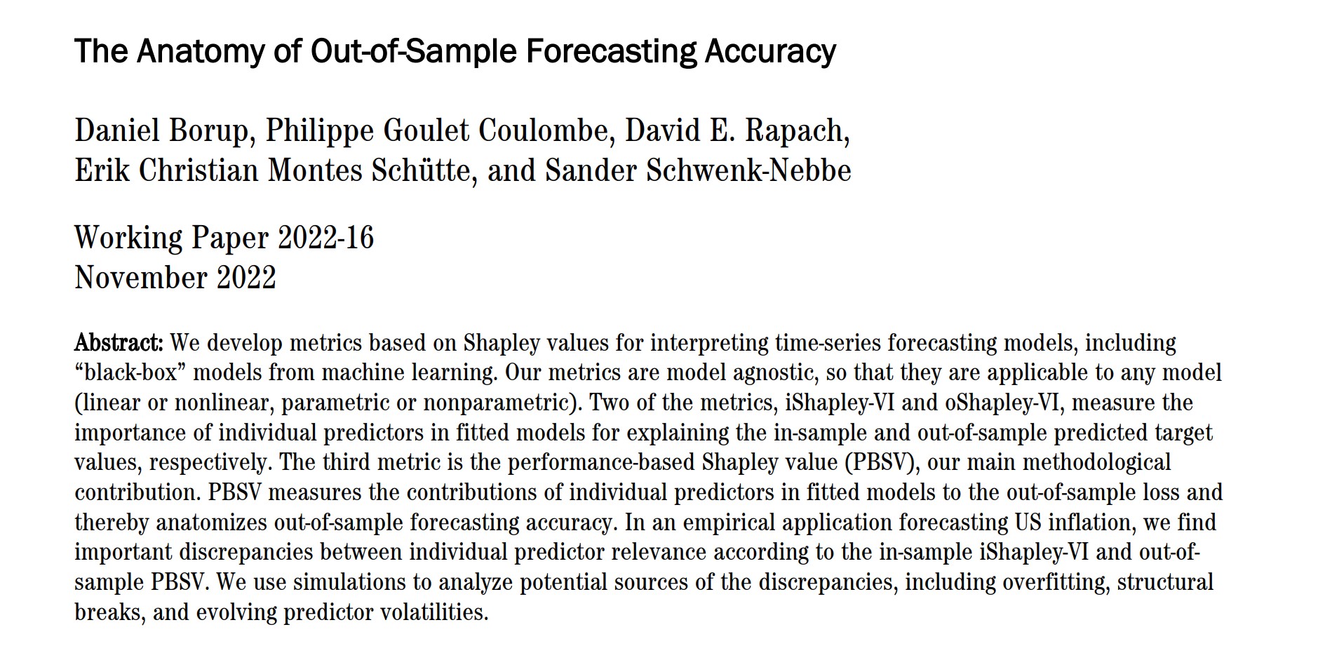
We have just released the paper The Anatomy of Out-of-Sample Forecasting Accuracy, which is joint work with Dave Rapach, Erik Christian Montes Schütte, Philippe Goulet Coulombe, and Daniel Borup.

In the paper, we develop performance-based Shapley values (PBSVs) to decompose the out-of-sample accuracy of a forecasting application. We provide the example application of forecasting US inflation with an ensemble of machine learning models, assess the accuracy with the RMSE (root mean squared error), and use PBSVs to allocate the RMSE between our predictors. The PBSVs tell us exactly how each individual predictor increased or decreased the final RMSE, thereby anatomizing out-of-sample forecasting accuracy.

We often want to understand how a given method, especially if it is new, works on something simple, before we apply it to something complex (like an ensemble of machine learning models). In this blog post, I give the example of a single-period forecasting problem and use OLS to estimate the parameters in a linear regression model with two predictors: \[ \hat{y}_{t+1}=\hat{\alpha}^{\text{OLS}}_t + \hat{\beta}^{\text{OLS}}_{1,t} x_{1,t} + \hat{\beta}^{\text{OLS}}_{2,t} x_{2,t} ~. \]

We want to know how well our model fares in predicting the target. For a single-period forecast, we would typically use the squared error loss function: \[\ell_{t+1}^{\text{SE}}=(y_{t+1}-\hat{y}_{t+1})^2~,\] but how would we go about allocating this loss between our two predictors?

Shapley Values

Shapley (1951) shows that we can gauge the value of player $p$ in a coalitional game of $P$ players by computing: \[ \phi_p=\sum_{Q\,\subseteq\,S\setminus\left\{p\right\}}\frac{\left|Q\right|!\left(P-\left|Q\right|-1\right)!}{P!}\left[v(Q\,\cup\,\{p\})-v(Q)\right] ~,\] where $S\setminus\left\{p\right\}$ is the set of all possible coalitions of players excluding $p$. The above is perhaps easiest to digest in its equivalent form: \[\phi_p=\frac{1}{P!}\sum_{\mathcal{O}\,\in\,\pi\left(P\right)}\left[v(\text{Pre}_p\left(\mathcal{O}\right)\,\cup\,\left\{p\right\})-v(\text{Pre}_p\left(\mathcal{O}\right))\right]~, \] where $\pi\left(P\right)$ is the set of all $P!$ possible permutations of $P$, and $\text{Pre}_p\left(\mathcal{O}\right)$ is the set of players that precede $p$ in $\mathcal{O}$. In words: to compute the value of a single player $p$ in a game with $P$ players, we need to evaluate the $P!$ possible ways in which the player can be added into the game, each time gauging by how much the value $v(\cdot)$ changes by the addition. The value that $p$ adds to the game is the simple average over the $P!$ marginal contributions.

We can apply the logic of Shapley values to our example. We can view our simple forecasting application as a coalitional game in which two predictors participate and ultimately produce the value \[v(S)=\ell_{t+1}^{\text{SE}}~,\] where $S$ is the set of all predictors. Because the value function is now related to the performance of the model, we call the resulting Shapley value a performance-based Shapley value (PBSV) and denote it by $\theta$.

Efficiency

Shapley values, including PBSVs, fulfill a number of desirable properties including efficiency, which states that the sum of the Shapley values yields the decomposed value exactly. In our example with two predictors, this means that: \[ \ell^{\text{SE}}_{t+1} = \theta_\emptyset(\ell_{t+1}^{\text{SE}}) + \theta_1(\ell_{t+1}^{\text{SE}}) + \theta_2(\ell_{t+1}^{\text{SE}})~, \] where $\theta_\emptyset(\ell_{t+1}^{\text{SE}})$ is the loss of the empty model given by \[ (y_{t+1} – \phi_{\emptyset,t})^2~,\] where $\phi_{\emptyset,t}$ is the naïve forecast, which for OLS is the average of the target the model was estimated on, typically denoted $\bar{y}$.

To compute the PBSV of predictor $p$ in our example, we need to introduce $p$ into the model in the two ($P!=2$) possible ways: into the empty model and into the model with predictor $q\neq p$ already present. This evaluates to: \[ \theta_p(\ell_{t+1}^{\text{SE}}) = \frac{1}{2}\left[ ( a_{+} – a_{-} ) + ( b_{+} – b_{-} ) \right]~, \] where $a_{-}$ is the squared loss of the empty model, $b_{-}$ is the squared loss of the model with $q \neq p$ present, and $a_{+}$ and $b_{+}$ is that same loss after including $p$ into the model.

General Solution

In The Anatomy of Out-of-Sample Forecasting Accuracy, we derive a closed-form solution for a linear model (with no interactions), the squared error, and any number of predictors. The PBSV of predictor $p$ evaluates to: \[ \theta_p(\ell_{t+1}^{\text{SE}}) = \phi_{p,t} \left[ (\hat{y}_{t+1}-y_{t+1}) – (y_{t+1}-\phi_{\emptyset,t}) \right] ~, \] where $\phi_{p,t}$ is the Shapley value of $p$ with regard to the forecast and $\phi_{\emptyset,t}$ is the naïve forecast of the model, the forecast of the empty set of predictors.

In words: the PBSV of the squared error of predictor $p$ in a linear model is proportional to the forecast error of the full model adjusted for the naïve forecast, where the factor of proportionality is the Shapley value of the forecast of predictor $p$, i.e., by how much the forecast is changing when $p$ is introduced into the model.

Is the Shapley-way of allocating the loss meaningful?

First, consider only the first part of the allocation, $\phi_{p,t}(\hat{y}_{t+1}-y_{t+1}) $. When our forecast is lower than the target value but $\phi_{p,t}>0$ then predictor $p$ is not to blame and is rewarded with $\theta_p(\ell_{t+1}^{\text{SE}})<0$. Conversely, if our forecast is higher than the target value and $\phi_{p,t}>0$, then the predictor nudged the forecast further away from the target and is penalized with $\theta_p(\ell_{t+1}^{\text{SE}})>0$.

Next, consider only the other part of the allocation, $-\phi_{p,t}(y_{t+1}-\phi_{\emptyset,t}) $. We penalize $p$ if it nudges the forecast further away from the target relative to the naïve forecast. If $p$ increases the forecast while the naïve forecast is above target, or if $p$ lowers the forecast while the naïve forecast is below target, then $\theta_p(\ell_{t+1}^{\text{SE}})>0$.

Consider now the full allocation and a perfect forecast. The allocation depends only on the naïve forecast because $\hat{y}_{t+1}-y_{t+1}=0$. If $\phi_{p,t}>0$ while the naïve forecast is below target, a reduction in loss is attributed to $p$ with $\theta_p(\ell_{t+1}^{\text{SE}})<0$.

However, if $\phi_{p,t}<0$, then $p$ is penalized with $\theta_p(\ell_{t+1}^{\text{SE}})>0$. The forecast is still perfect, but this cannot be attributed to predictor $p$ because this predictor contributed to the forecast being lower than the naïve forecast and further away from the target. Other predictors will be credited instead. That is, the perfect forecast with naïve forecast below target implies that there are other predictors $q \neq p$ with $\phi_{q,t}>0$ that are rewarded with $\theta_q(\ell_{t+1}^{\text{SE}})<0$ because they nudged the forecast above the naïve forecast, ultimately producing the perfect forecast.

References:

[1] Shapley, Lloyd S. (1951). “Notes on the n-Person Game — II: The Value of an n-Person Game”. Santa Monica, Calif.: RAND Corporation.

[2] Borup, Daniel and Coulombe, Philippe Goulet and Rapach, David E. and Montes Schütte, Erik Christian and Schwenk-Nebbe, Sander (2022). “The Anatomy of Out-of-Sample Forecasting Accuracy”. Federal Reserve Bank of Atlanta Working Paper 2022-16. https://doi.org/10.29338/wp2022-16. Available at SSRN: https://ssrn.com/abstract=4278745.

$$ $$